Tutorial
This section guides you through a tutorial for an example model and usage pattern of SPUX. For peculiarities regarding the coupling your model with the SPUX framework, refer to Customization.
Overview
Commands should be executed in Python terminal, or inside a Python script, or in a Jupyter notebook. To learn how to write your own custom scripts and configure spux, first read through the rest of this section and take a look at the examples suite.
Editor
Try one of the following cross-platform editors (you can also use Vim or Emacs, of course):
- Spyder - similar UI as R,
- PyCharm - proprietary,
- VS Code - works very well with GitLab integration extensions - give it a try!
Model stochasticity
SPUX supports two types of models for the Bayesian inference:
- Deterministic - model evaluation is uniquely determined by the inputset and parameters,
- Stochastic - model evaluation is additionally driven by a random variable/process.
Bayesian inference of model parameters for deterministic models is often less difficult,
since a simple so-called Direct likelihood can be used,
which, for any given parameters, is analytically computed from the specified error model.
Error model describes a probabilistic distribution for observational data,
conditional on the true model evaluation (referred to as model prediction).
For stochastic models, in addition to uncertain model parameters, also the uncertain model evaluations (predictions, sometimes referred to as states) need to be inferred. To this end, the error model alone is often not sufficient to analytically compute the marginal likelihood of a given dataset and model parameters. Currently SPUX supports the Particle Filter approximation of such marginal likelihood, used in this tutorial.
As SPUX framework has a focus on the Bayesian inference in stochastic models,
in the present tutorial we also focus on the stochastic models, with an example of a Randomwalk.
Straightwalk is another educational model available in SPUX,
which is simply a stripped down version (with the randomness eliminated) of the stochastic Randomwalk model.
To learn more about the Straightwalk and how to use SPUX with deterministic models,
we recommend to read the tutorial below and then
refer to analogous example scripts in the respective example directory at:
examples/straightwalk/.
Replicate datasets
In some applications, multiple replicates of observational datasets are available, with each replicate dataset corresponding to the same (assumed to be unknown) model parameter values, but different independent stochastic model evaluations (for instance, w.r.t. the seed of the pseudo-random number generator.) Examples of such replicates could be independent datasets from several consecutive sufficiently separated time periods, or even several simultaneously collected measurements from independent experimental sites.
If this is the case, each dataset (and the respective model inputset) can be treated statistically independently
but at the same time fully integrated into the SPUX framework by simply merging
individual respective (direct or marginal) likelihoods into a single Replicates likelihood.
For the sake of simplicity, this tutorial only considers a single dataset.
To learn more about how to use SPUX with multiple independent replicate datasets,
we recommend to read the tutorial below and then
refer to analogous example scripts in the respective example directory at:
examples/randomwalk-replicates/.
Randomwalk (serial)
Here we provide an elaborate description of the SPUX framework setup and simulation execution for an example of a simple Randomwalk model.
Model description
The model describes a stochastic one-dimensional walk on integers,
with a prescribed (let’s say, genetically) stepsize.
Starting at the location given by the origin parameter,
a randomwalk takes a random step of size stepsize either to the left or to the right,
with direction distribution depending on the drift parameter.
Inaccurate observations at several times of the randomwalk’s position are available,
with unknown observational error distribution,
assumed to be Gaussian with zero mean and standard deviation given by the parameter $\sigma$.
All files required throughout this example (and some more) could be found in
examples/randomwalk/,
which we assume is the current working directory where commands are executed.
This means that all import module statements will import the corresponding module.py script from this directory (or an already installed external Python module).
All imports starting with from spux import ... import modules that are built-in in the spux module,
and we use relative links starting with spux/ for a corresponding file in the GitLab repository.
The randomwalk model is a built-in module in spux and can be found at spux/models/randomwalk.py:
from scipy import stats
import numpy

from spux.models.model import Model
from spux.utils.annotate import annotate

class Randomwalk (Model):
    """Class for Randomwalk model."""

    # no need for sandboxing
    sandboxing = 0

    # construct model
    def __init__ (self, stepsize=1):

        self.stepsize = stepsize

    # initialize model using specified 'inputset' and 'parameters'
    def init (self, inputset, parameters):
        """Initialize model using specified 'inputset' and 'parameters'."""

        # base class 'init (...)' method - OPTIONAL
        Model.init (self, inputset, parameters)

        self.position = parameters ["origin"]
        self.drift = parameters ["drift"]

        self.time = 0

    # run model up to specified 'time' and return the prediction
    def run (self, time):
        """Run model up to specified 'time' and return the prediction."""

        # base class 'run (...)' method - OPTIONAL
        Model.run (self, time)

        # pre-generate random variables for all steps
        steps = time - self.time
        distribution = stats.uniform (loc=-1, scale=2)
        rvs = distribution.rvs (steps, random_state=self.rng)

        # update position (e.g., perform walk)
        directions = numpy.where (rvs < self.drift, 1, -1)
        self.position += self.stepsize * numpy.sum (directions)

        # update time
        self.time = time

        # return results
        return annotate ([self.position], ['position'], time)
In the source code above, Randomwalk class has a constructor (note the underscores!) __init__ (self, ...),
which is called when constructing model by model = Randomwalk (stepsize=1).
The argument self is a pointer to the object itself, analogous to this in C/C++.
Additional methods include:
init (self, inputset, parameters)- initialize model with the specifiedinputsetandparameters,run (self, time)- run model from the current time up to the specifiedtime.
Note, that the “current time” in the above is set in init (...) or the previous call of run (...)
and is handled differently in different models (in this example: simply saving it to self.time).
The annotate (values, labels, time) method packages model predictions stored in values to a pandas.DataFrame
with the specified list of labels for the elements if the values and with the requested time.
SPUX configuration
Apart from the actual model, we also need to specify several auxiliary configuration files for observational datasets, statistical error model (i.e. a probabilistic distribution of the observations conditional on the specified model prediction), and prior distribution of the parameters. Actual dataset files are located in the datasets directory at examples/randomwalk/datasets/.
The script to load the dataset into pandas DataFrames (a default container for dataset management in SPUX, see https://pandas.pydata.org) is located in
examples/randomwalk/dataset.py.
import pandas
dataset = pandas.read_csv ('datasets/dataset.dat', sep=",", index_col=0)
Error model is defined in
examples/randomwalk/error.py
as an object with a method distribution (prediction, parameters)
which returns a distribution of the model observations (dataset):
from scipy import stats
from spux.distributions.tensor import Tensor

# define an error model
class Error (object):

    # return an error model (distribution) for the specified prediction and parameters
    def distribution (self, prediction, parameters):

        # specify error distributions using stats.scipy for each observed variable independently
        # available options (univariate): https://docs.scipy.org/doc/scipy/reference/stats.html
        distributions = {}
        distributions ['position'] = stats.norm (prediction['position'], parameters[r'$\sigma$'])

        # construct a joint distribution for a vector of independent parameters by tensorization
        distribution = Tensor (distributions)

        return distribution

error = Error ()
Prior distribution is defined in examples/randomwalk/prior.py:
# specify prior distributions using stats.scipy for each parameter independently
# available options (univariate): https://docs.scipy.org/doc/scipy/reference/stats.html

from scipy import stats

from spux.distributions.tensor import Tensor
from spux.utils import transforms

distributions = {}

distributions ['origin'] = stats.uniform (loc=50, scale=100)
distributions ['drift'] = stats.uniform (loc=-1, scale=2)
distributions [r'$\sigma$'] = stats.lognorm (**transforms.logmeanstd (logm=10, logs=1))

# construct a joint distribution for a vector of independent parameters by tensorization
prior = Tensor (distributions)
Within the context if this illustrative Randomwalk example, we also make use of the (optional) exact (“the truth”)
parameter values as well as the model predictions (without the observational noise) which are set at
examples/randomwalk/exact.py:
# exact parameters
parameters = {}
parameters ['origin'] = 100
parameters ['drift'] = 0.2
parameters [r'$\sigma$'] = 10

# exact predictions
import os, pandas
filename = 'datasets/predictions.dat'
if os.path.exists (filename):
    predictions = pandas.read_csv (filename, sep=",", index_col=0)
else:
    predictions = None

# dictionary for exact parameters and predictions
exact = {'parameters' : parameters, 'predictions' : predictions}
The datasets (and the predictions) in the examples/randomwalk/datasets/ directory were generated using the above exact model parameters from examples/randomwalk/exact.py by the synthesis script based on the built-in SPUX data generation method: examples/randomwalk/script_synthesize.py
from spux.models.randomwalk import Randomwalk
from exact import exact
from error import error

model = Randomwalk ()
parameters = exact ['parameters']
steps = 1000
period = 20
times = range (period, period + steps, period)

sandbox = None

from spux.utils.seed import Seed
seed = Seed (2)

from spux.utils import synthesize
synthesize.generate (model, parameters, times, error, sandbox = sandbox, seed = seed)
We would also like to emphasize, that in the above scripts we generously use LaTeX syntax
within labels for parameters, predictions, and observations.
The benefit of such scrupulous naming will become evident from the generated plots
within this tutorial, where all axes labels are LaTeX-formatted mathematical symbols.
Notice, that for a LaTeX syntax to be supported in Python,
one must prepend the string with the r letter (as in “raw”).
In order to give you a better overview of the datasets, the error model, the prior distribution, and (optional) exact parameters values for a reference, consider running a preparation script examples/randomwalk/plot_config.py:
# generate config
import script
del script

# plotting class
from spux.plot.mpl import MatPlotLib
from exact import exact
plot = MatPlotLib (exact = exact)

# plot dataset
plot.dataset ()

# plot marginal prior distributions
plot.priors ()

# plot marginal error model distributions
plot.errors ()

# generate report
from spux.report import generate
generate.report (authors = r'Jonas {\v S}ukys')
The above script plots model observations (datasets),
marginal prior distributions of model parameters,
and marginal error model distributions for specified model prediction and parameters
and by default saves them in the fig directory under multiple file formats (PDF, EPS, SVG, PNG),
additionally including a caption file *.cap containing the description of the figure contents:

Observational dataset.
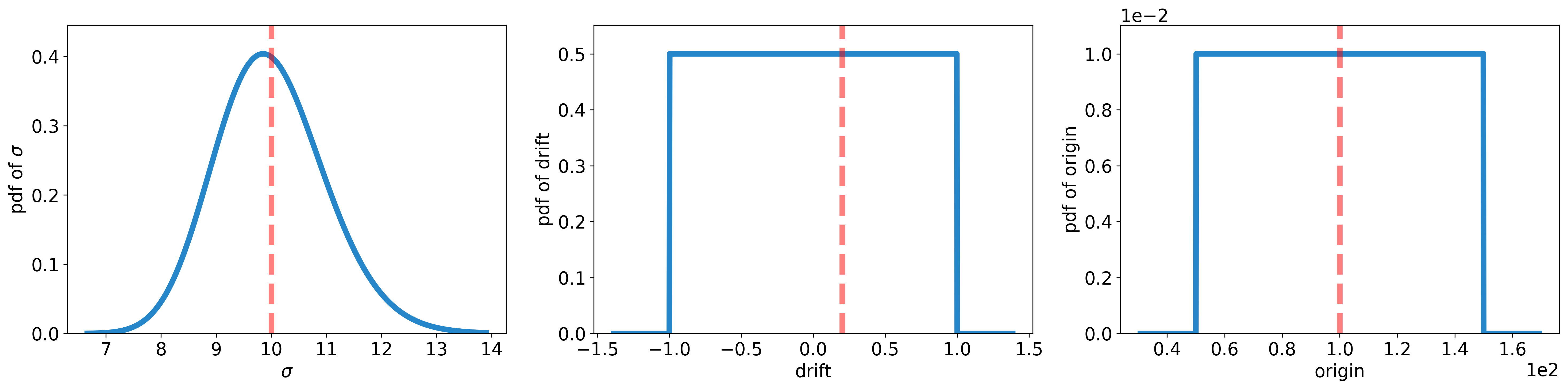
Marginal distributions (prior).

Observational dataset and the associated error model, evaluated using exact model predictions and exact model parameters. The circles (or thick dots) indicate the dataset values, the thick solid line indicates the model predictions used in the error model. The shaded green regions indicate the density of the error model distribution.
In addition to the plots,
an auxiliary report directory is created
(can be changed by setting reportdir in sampler.setup (...)),
including information regarding SPUX framework setup.
Each report file in the report directory is saved using three different formats:
.dat- a (cloudpickle) binary dump of the respective Python object or dictionary,.txt- a formatted ASCII table to be easily read directly,.tex- a formatted LaTeX table to be included in a LaTeX report..cap- a caption with the table title and description of the table contents.
At the end of the plot_config.py script all generated plots are compiled into a LaTeX report under directory latex,
where a PDF report is also generated if the pdflatex can be found in the system (which is not a SPUX dependency).
The PDF report for this example can be downloaded here.
The report is continuously overwritten with the newest plots and tables,
and contains separate sections for the SPUX framework setup, and, as described in the following sections,
the results of the inference run and the computational performance amd runtime profiling reports.
As already hinted in the report above, the main script examples/randomwalk/script.py, uses the above auxiliary scripts to configure SPUX:
# === Randomwalk model

# construct Randomwalk model
from spux.models.randomwalk import Randomwalk
model = Randomwalk (stepsize = 1)

# === SPUX

# LIKELIHOOD
# for marginalization in stochastic models, construct a Particle Filter likelihood
from spux.likelihoods.pf import PF
likelihood = PF (particles = [4, 8], threshold=-5)

# SAMPLER
# construct EMCEE sampler
from spux.samplers.emcee import EMCEE
sampler = EMCEE (chains = 8)

# ASSEMBLE ALL COMPONENTS
from error import error
from dataset import dataset
from prior import prior
likelihood.assign (model, error, dataset)
sampler.assign (likelihood, prior)
In this script, different additional components, such as model, likelihood, and sampler, are created.
Afterwards, all these components are merged together by assigning according to the logical dependencies.
In the future, SPUX will provide a spux.utils.assign module containing a assign function,
which takes a list of components (in any order) as an argument, tries to “automagically” perform all needed assignments
(assuming all components are directly derived from the respective SPUX component base classes)
and returns the resulting top-level component (in this example, the sampler):
from spux.utils.assign import assign
components = [model, error, dataset, likelihood, prior]
sampler = assign (sampler, components)
The corresponding SPUX configuration table from report/randomwalk_config.txt reports
the selected class for each SPUX component, together with the selected constructor arguments:
===================================================================================================================================
SPUX components configuration
===================================================================================================================================
Component  | Class      | Options
---------- + ---------- + ---------------------------------------------------------------------------------------------------------
Model      | Randomwalk | stepsize=1
Likelihood | PF         | particles=[4, 128], adaptive=True, accuracy=0.1, margin=0.05, threshold=-5, factor=2, log=1, noresample=0
Sampler    | EMCEE      | chains=8, a=2.0, attempts=100, reset=10
===================================================================================================================================
In the SPUX configuration above, in the constructor arguments of the PF marginal likelihood estimator,
the number of particles, instead of being a fixed number,
is set to a list indicating the minimum and maximum number of particles to be used adaptively,
starting with the minumum number of particles and then iteratively
taking into account the feedback from the empirical standard deviations of these estimates.
SPUX results
It is a good idea to keep this main script.py separate from the scripts that will actually run SPUX,
in order to have flexibility for the later customization of output location, sampling duration, and the targeted hardware resources.
To achieve this, we import the main configuration script and initiate the execution of the framework in a separate script named (you will see later why such name) examples/randomwalk/script_serial.py:
# === SCRIPT

from script import sampler

# === SAMPLING

# SANDBOX
# use fast tmpfs
from spux.utils.sandbox import Sandbox
sandbox = Sandbox (path = None, target = '/dev/shm/spux-sandbox')

# SEED
from spux.utils.seed import Seed
seed = Seed (8)

# init executor
sampler.executor.init ()

# setup sampler
sampler.setup (sandbox = sandbox, verbosity = 1, seed = seed, lock = 50)
#sampler.setup (sandbox = sandbox, verbosity = 1, seed = seed, lock = 50, thin = 4)

# init sampler (use prior for generating starting values)
sampler.init ()

# generate samples from posterior distribution
sampler (12)

# exit executor
sampler.executor.exit ()
Within sampler.setup (...), various additional (optional) sampling options can be set, including:
sandboxinstance - target filesystem and directory for the SPUX sandbox,verbosity- [0 to infinity] limits the depth of verbosity in the hierarchy of SPUX components,seedinstance - initial seed array for the pseudo random number generators,lock- batch index to lock sampler’s feedback to likelihood (e.g. adaptivePF) [default:None],thinperiod - to save only everythin-th sample batch and information [default:None].
The adaptive number of particles in PF is meant to be used only during the initial burn-in period,
after which, if the number of particles is not completely stationary, the adaptation should be locked.
The optional lock argument in the sampler.setup (...) can be used
to stop the adaptation of the number of particles in PF and lock the most recent value until the end of sampling.
The sandbox in this example script is configured to use the fast virtual node-local RAM-based Linux filesystem called tmpfs.
Note, that the exact path to the local tmpfs might differ depending on the Linux distribution.
For local testing, a user might prefer to temporarily switch to a conventional filesystem and set a different desired sandbox path, leaving target=None.
For production runs on high performance computing clusters, we recommend either to use the default tmpfs,
or, if the amount of system memory is a limiting factor, to set target to the scratch file system of the cluster.
Node-local (not shared) scratch filesystems are preferable, due to their better performance and the lack of restrictions regarding any storage quotas.
If target is a shared (hence not a node-local) filesystem (the worst case scenario, for development only), you can also set path, where a corresponding symlink pointing to the specified target will be created.
Regarding the auxiliary calls sampler.executor.init () and sampler.executor.exit (),
you must have them, and in this particular order, i.e. wrapping every other call of the SPUX framework
(apart from the calls in the main configurations script).
The main script then generates an output/ directory
(can be changed by setting outputdir in sampler.setup (...))
with files containing posterior samples and supporting information;
multiple files of each type will be generated for each checkpoint,
with the default period being 10 minutes:
samples-*.csv- a CSV file containing comma-separated posterior samples of parameters,samples-*.dat- a binary file (cloudpickle) containing posterior samples of parameters,infos-*.dat- a binary file (cloudpickle) containing alistof supporting information,pickup-*.dat- a binary file (cloudpickle) containing a dictionary of sampler pickup information.
The supporting files infos-*.dat contain detailed information about
each component in the hierarchical assignment structure specified by the main configuration script.
In the particular example, when loaded (see following paragraphs) will contain a list of dictionaries for each draw of the posterior parameters from the sampler.
For samplers supporting multiple MCMC chains, each draw provides as many samples as there are chains,
and hence the list in the infos-*.dat will be shorter than the list of all posterior parameters by a factor of the number of chains.
The structure of each element in the list of loaded infos-*.dat can be inferred from the corresponding info generation routines for each SPUX component (look for info = {...}).
The sampler pickup files pickup-*.dat contain all information
needed to continue sampling past the respective checkpoint
(will be discussed in detail in the following sections).
In addition to the output directory, the auxiliary report directory is also updated,
appending information regarding
computational environment (in report/randomwalk_environment.txt):
=============================================================
Computational environment
=============================================================
Descriptor         | Value
------------------ + ----------------------------------------
Timestamp          | 2019-05-23 00:58:01
Version            | 0.3.0
GIT branch (plain) | dev_jonas
GIT revision       | f98e24ae81841a98a39d7d9e3b655ae6cdc97d4f
=============================================================
required computational resources (in report/randomwalk_resources.txt):
============================================================================================
Required computational resources
============================================================================================
Component  | Class      | Task       | Executor | manager | workers | resources | cumulative
---------- + ---------- + ---------- + -------- + ------- + ------- + --------- + ----------
Model      | Randomwalk | -          | -        |       0 |       1 |         1 |          1
Likelihood | PF         | Randomwalk | Serial   |       0 |       1 |         1 |          1
Sampler    | EMCEE      | PF         | Serial   |       0 |       1 |         1 |          1
============================================================================================
sampler setup (in report/randomwalk_setup.txt):
==========================================
Setup argument list
==========================================
seed | thin | lock (batch) | lock (sample)
---- + ---- + ------------ + -------------
[8]  | None | 100          | 800
==========================================
the cumulative number of model evaluations in each SPUX component (in report/randomwalk_evaluations.txt):
====================================================
Number of model evaluations
====================================================
Component  | Class      | tasks | sizes | cumulative
---------- + ---------- + ----- + ----- + ----------
Model      | Randomwalk |    1  |    1  |         1
Likelihood | PF         |  128  |    1  |       128
Sampler    | EMCEE      |    1K |  128  |       128K
====================================================
and the structure of the information available in infos-*.dat:
======================================================================================================================================================================================================================
SPUX infos structure
======================================================================================================================================================================================================================
Component  | Class | Fields                                                                                                                                                                      | Iterators for infos
---------- + ----- + --------------------------------------------------------------------------------------------------------------------------------------------------------------------------- + -------------------
Sampler    | EMCEE | proposes, infos, parameters, posteriors, accepts, likelihoods, timing, priors, timings, index, feedbacks, feedback, resets                                                  | 0 - 8
Likelihood | PF    | particles, successful, variances, sources, timing, MAP, timings, redraw, weights, predictions_prior, estimates, variance, errors_prior, predictions, traffic, avg_deviation | -
======================================================================================================================================================================================================================
If self.sandboxing == 1 is set for the model,
a sandbox directory is created (or a custom name, if custom sandbox is specified).
This directory is populated with nested sandboxes for each sample, chain, replicate, likelihood, and model.
For sandboxes in the local mode (for non-shared filesystems), nested directories are replaced by a single directory with a long name indicating the underlying hierarchy.
Please also note, that sandboxes in local mode are tentative, meaning that they are only created once self.sandbox () is executed for the first time.
If trace=True is additionally specified in the sampler.setup (...),
this directory contains the stored sandboxes of all samplers,
likelihoods and models, including all the generated results. However, these results would be easily accessible only if sandboxes are placed in a shared filesystem and a non-local mode is used.
In the future, SPUX will explicitly save the sandbox with a complete trace of the model output
(independently of the value set to trace)
for the approximated joint maximum a posteriori (MAP) model parameters and states
under the directory specified in sampler.setup (...) by MAPdir with the default being 'MAP'.
In addition, there will be an option to save only a (possibly thinned) collection
of posterior sandboxes by specifying trace = 'posterior' in sampler.setup (...).
An example analysis script to load and visualize results from the output/ directory is available at
examples/randomwalk/plot_results.py:
# === load results

from spux.io import loader
samples, infos = loader.reconstruct ()

# === plot

# burnin sample batch
burnin = 70

# plotting class
from spux.plot.mpl import MatPlotLib
from exact import exact
plot = MatPlotLib (samples, infos, burnin = burnin, exact = exact)

# plot unsuccessful posteriors
plot.unsuccessfuls ()

# plot resets of stuck chains
plot.resets ()

# compute and report approximated maximum a posterior (MAP) parameters estimate
plot.MAP ()

# plot samples
plot.parameters ()

# plot evolution of likelihoods
plot.likelihoods ()

# plot evolution of likelihood accuracies
plot.accuracies ()

# plot evolution of likelihood particles
plot.particles ()

# plot redraw rates
plot.redraw ()

# plot evolution of acceptances
plot.acceptances ()

# plot timestamps
plot.timestamps ()
timestamps = [ "evaluate", "routings", "wait"]
timestamps += [ "init", "init sync", "run", "run sync"]
timestamps += ["errors", "errors sync", "resample", "resample sync"]
plot.timestamps (keys = timestamps, suffix = '-cherrypicked')

# === remove burnin

samples, infos = loader.tail (samples, infos, batch = burnin)
plot = MatPlotLib (samples, infos, burnin = burnin, tail = burnin, exact = exact)
plot.MAP ()

# plot autocorrelations
plot.autocorrelations ()

# compute and report effective sample size (ESS)
plot.ESS ()

# plot marginal posterior distributions
plot.posteriors ()

# plot pairwise joint posterior distributions
plot.posteriors2d ()

# plot pairwise joint posterior distribution for selected parameter pairs
plot.posterior2d ('origin', 'drift')

# plot posterior model predictions including datasets
plot.predictions ()

# plot quantile-quantile comparison of the error and residual distributions
plot.QQ ()

# show metrics
plot.metrics ()

# generate report
from spux.report import generate
generate.report (authors = r'Jonas {\v S}ukys')
This script uses some built-in plotting routines available in spux/plot/mpl.py module.
However, the user is free to use only the loading parts and choose how to visualize the results using other established data visualization libraries,
including the built-in visualization module pandas.plotting in pandas for the visualization of the pandas.DataFrame objects.
Also check out NumFOCUS.
Note, that for runtime saving purposes, actual linked example scripts in repository usually could be setup for smaller computational resources (i.e. fewer particles, chains, samples, etc.), and hence the following example plots for SPUX results could differ from your versions (please check the corresponding entries in the provided configuration and setup tables above).
The above analysis script generates multiple plots of the results, but firstly it is most useful to look at the unsuccessfuls and resets plots.
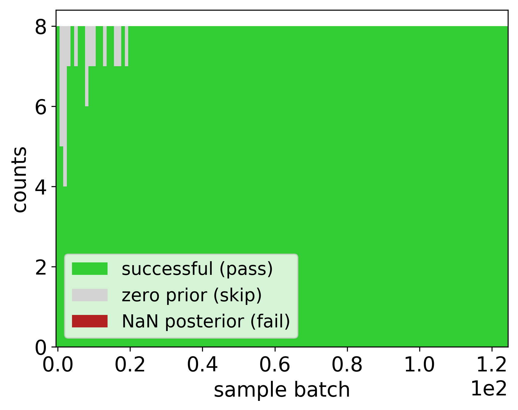
Diagnostics of the posterior sampler, indicating the successes and failures of the likelihood estmation procedures. Legend: green - successfully passed, gray - estimation skipped due to (numerically) zero prior, red - estimation failure due to failed model simulatios and/or failed PF filtering.
Note, that skipped likelihoods are not scheduled in the executor and might result in a temporary (for that particular parameter proposal) parallelization imbalances due to the lack of tasks to process.
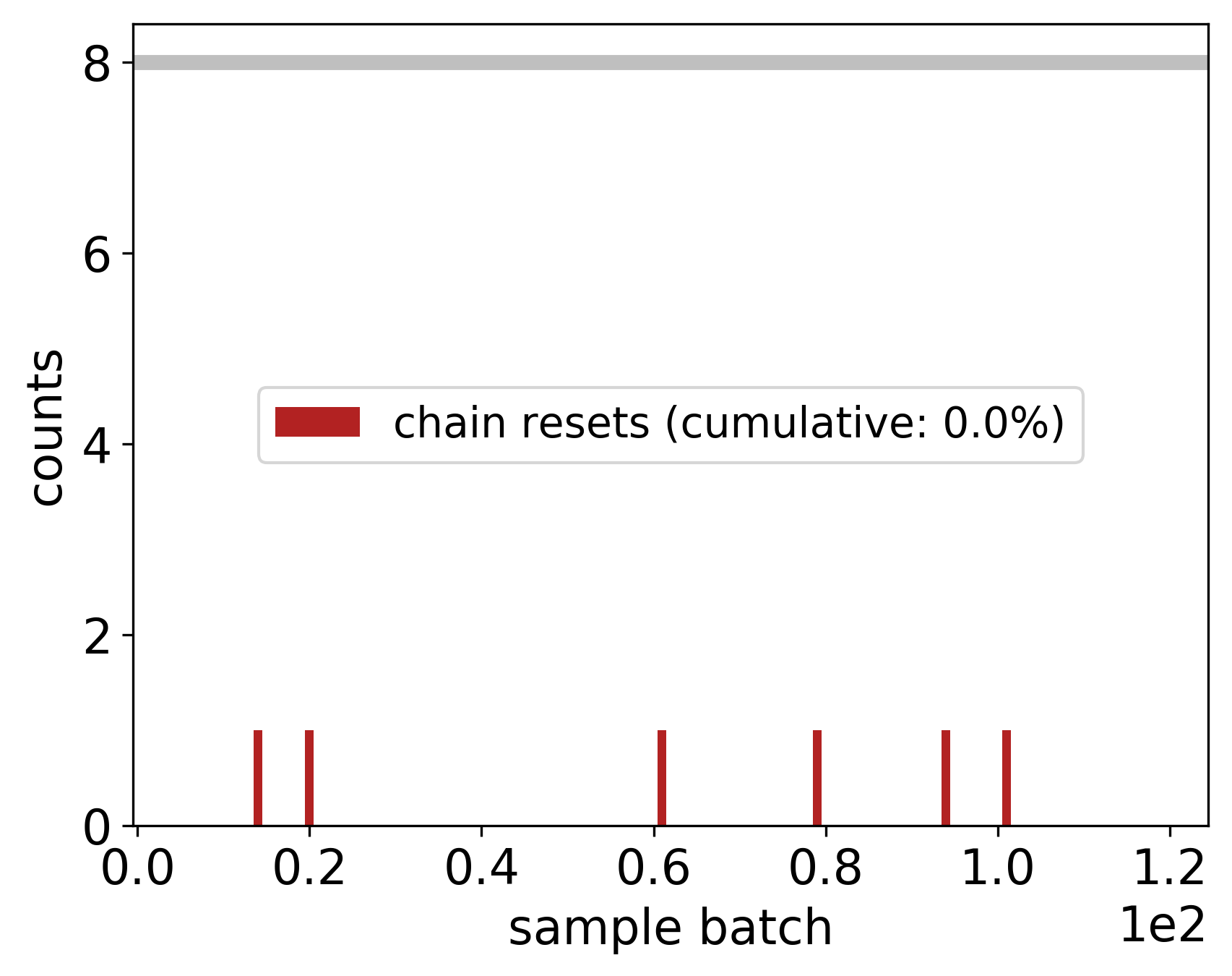
The report for the number of resets (re-estimation of the marginal likelihood) for stuck Markov chains, including the cumulative percentage of resets relative to the total number of samples.
From the diagnostic plot above, we determine that the inference was (tentatively) successful: not many failed (NaN) or skipped (zero prior) likelihood evaluations, and a negligible amount of total chain resets (likelihood re-estimations).
The next most important plots are the parameters plot, reporting the sampling progress of all sampler chains,

Markov chain parameters samples. The solid lines indicate the median and the semi-transparent spreads indicate the 5% - 95% percentiles accross multiple concurrent chains of the sampler. An auxiliary semi-transparent line indicates an example of such chain. The thick semi-transparent gray lines indicate the interval containing centererd 99% mass of the respective prior distribution. The brown dotted line indicates the estimated maximum a postriori (MAP) parameters values. The red dashed line represents the exact parameter values.
and the progress of the corresponding likelihood, accuracies, particles, redraw, and acceptances plots
providing diagnostic information of the algorithmic technicalilies within the PF likelihood estimation
and Markov chain sampling:
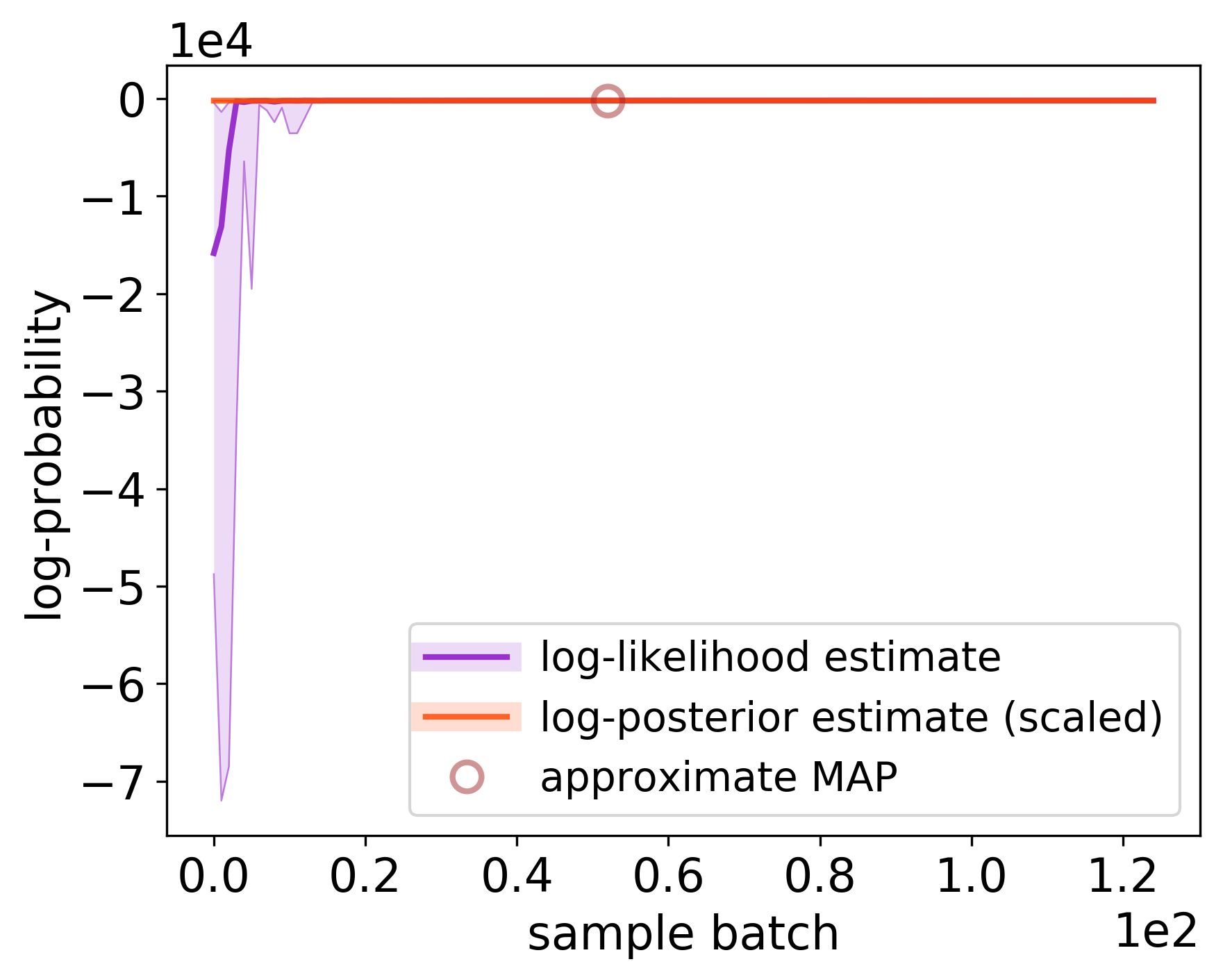
Log-likelihood and (scaled [TODO: estimate evidence and remove scaling]) log-posterior estimates for the sampled model posterior parameters. The solid lines indicate the median and the semi-transparent spreads indicate the 10% - 90% percentiles accross multiple concurrent chains of the sampler. For log-likelihood, the estimates from the rejected proposed parameters are also taken into account.The brown “o” symbol indicates the posterior estimate at the approximate MAP parameters.
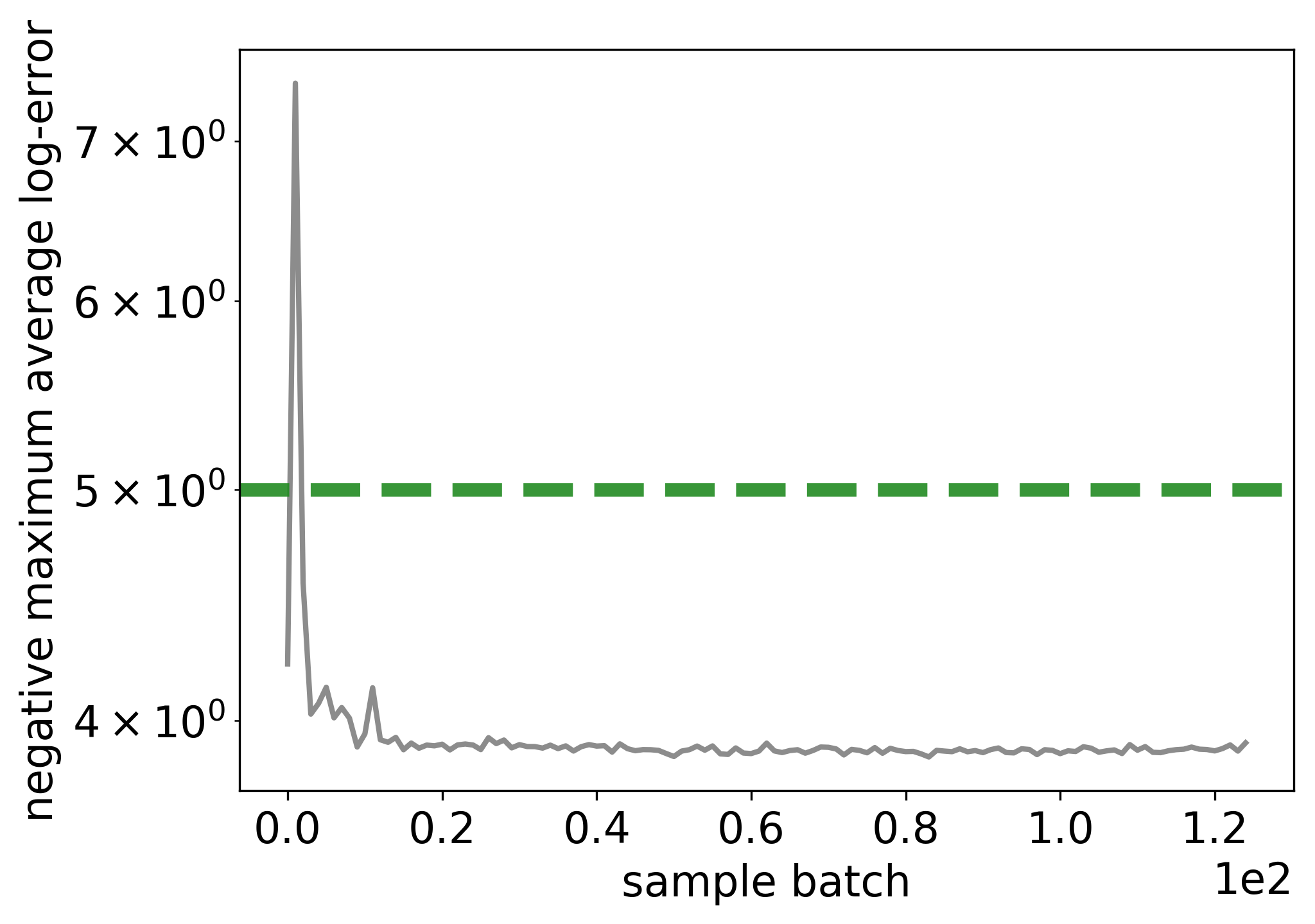
Maximums of the average (over dataset snapshots) marginal observational log-errors accross multiple concurrent chains of the sampler. The dashed green line indicates the threshold set in the adaptive PF likelihood.

Average (over dataset snapshots) standard deviations for the estimated marginal observational log-error using the PF. The semi-transparent spread indicates the range (minimum and maximumum) accross multiple concurrent chains of the sampler and the solid line indicates the value of the chain with the largest estimated log-likelihood. The solid thick gray line above the same line for a zero value reference indicates the specified accuracy and the dashed thick gray lines indicate the specified margins - all specified within the adaptive PF likelihood.
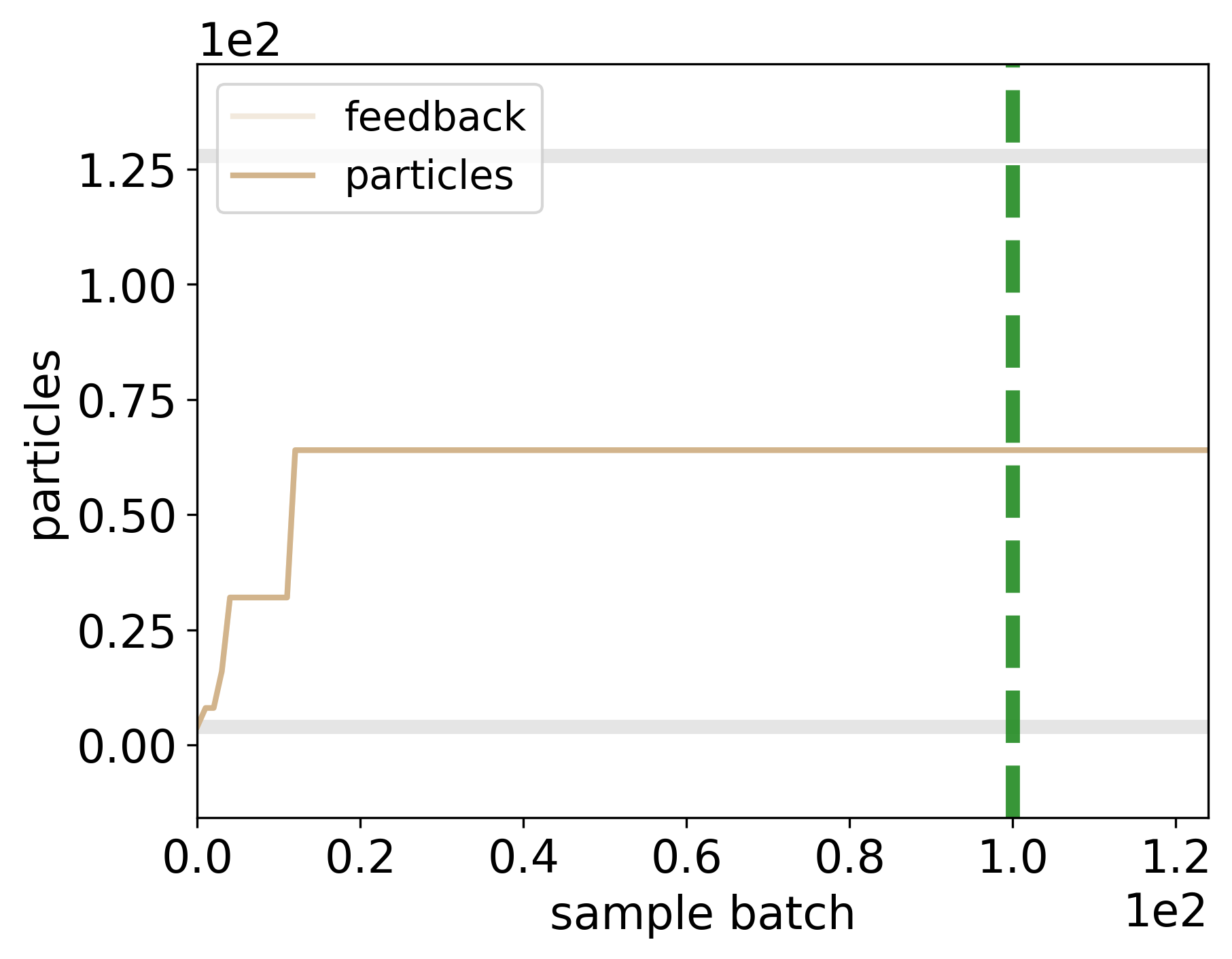
The adaptavity of the number of particles in the PF likelihood. The brighter line indicates the feedback (recommendation) of the adaptation algorithm, and the darker line indicates the actual number of used particles. The semi-transparent thick gray lines indicate the limits for minimum and the maximum number of allowed particles in the PF likelihood.
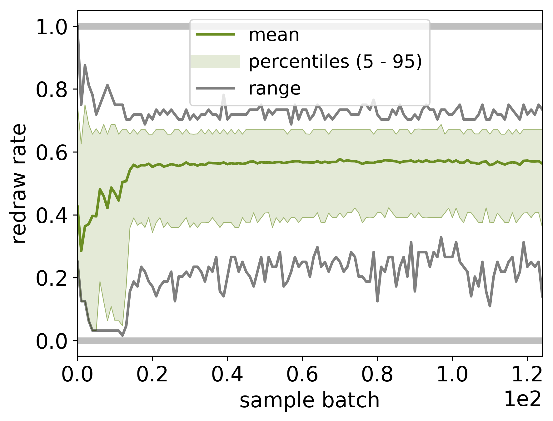
Particle redraw rates (the fraction of surviving particles) in the PF likelihood estimator. The solid line indicates the mean, the semi-transparent spreads indicate the 5% - 95% percentiles, and the dotted lines indicate the range (minimum and maximum) accross multiple concurrent chains of the sampler.
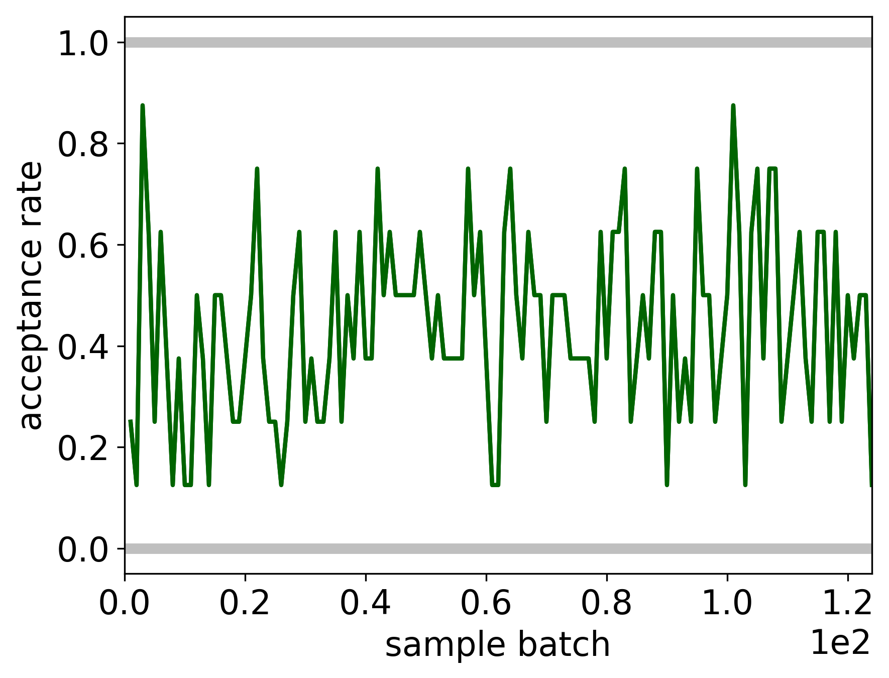
Acceptance rate (accross multiple concurrent chains of the sampler) for the proposed parameters samples.
We estimate the burnin period to last for approximately 70 batches of EMCEE samples from multiple chains.
We use this information to generate all subsequent plots with the initial bias already removed
by setting burnin=70 in the reconstruct method for loading results in the plot_results.py script above.
We note, that lock sample batch reported in the setup table above must not exceed the selected burnin
to ensure that the number of particles in PF likelihood is fixed throught the posterior sampling
(and hence avoid any potential bias due to the adaptivity process).
The resulting inference plots provide a detailed insight into posterior parameters and model predictions distributions,
as well as the performance of the overall Bayesian inference.

Marginal posterior (orange) and prior (blue) distributions of model parameters. The brown dotted line indicates the estimated maximum a postriori (MAP) parameters values. The red dashed line represents the exact parameter values.
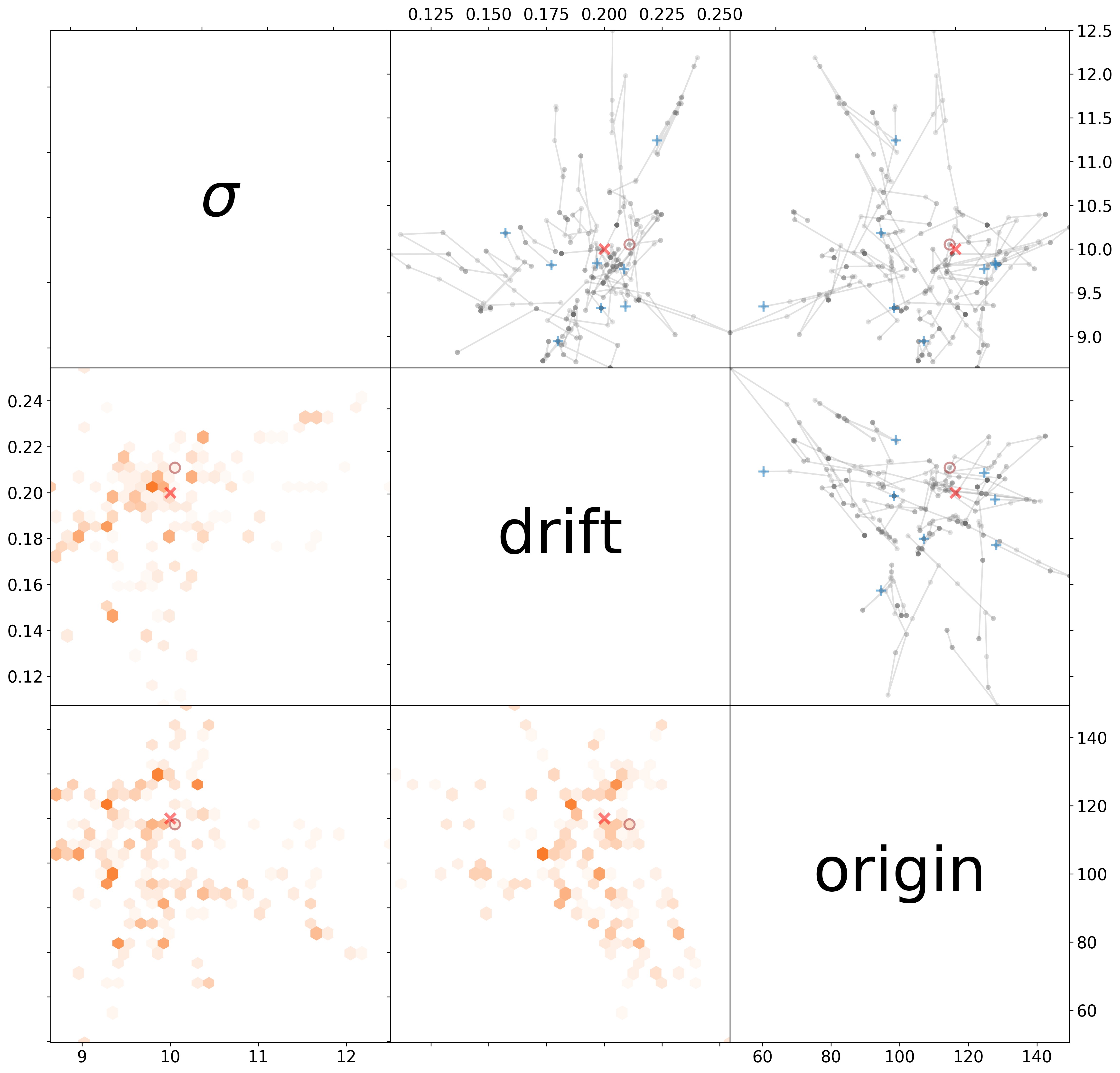
Joint pairwise marginal posterior distribution of all model parameters, including the corresponding Markov chains from the sampler. Legend: thick semi-transparent gray lines - intervals containing centererd 99% mass of the respective prior distribution, blue “+” - initial parameters, brown “o” - approximate MAP parameters, red “x” - the exact parameters, thin semi-transparent gray lines and dots - concurrent chains, orange hexagons - histogram of the joint pairwise marginal posterior parameters samples.
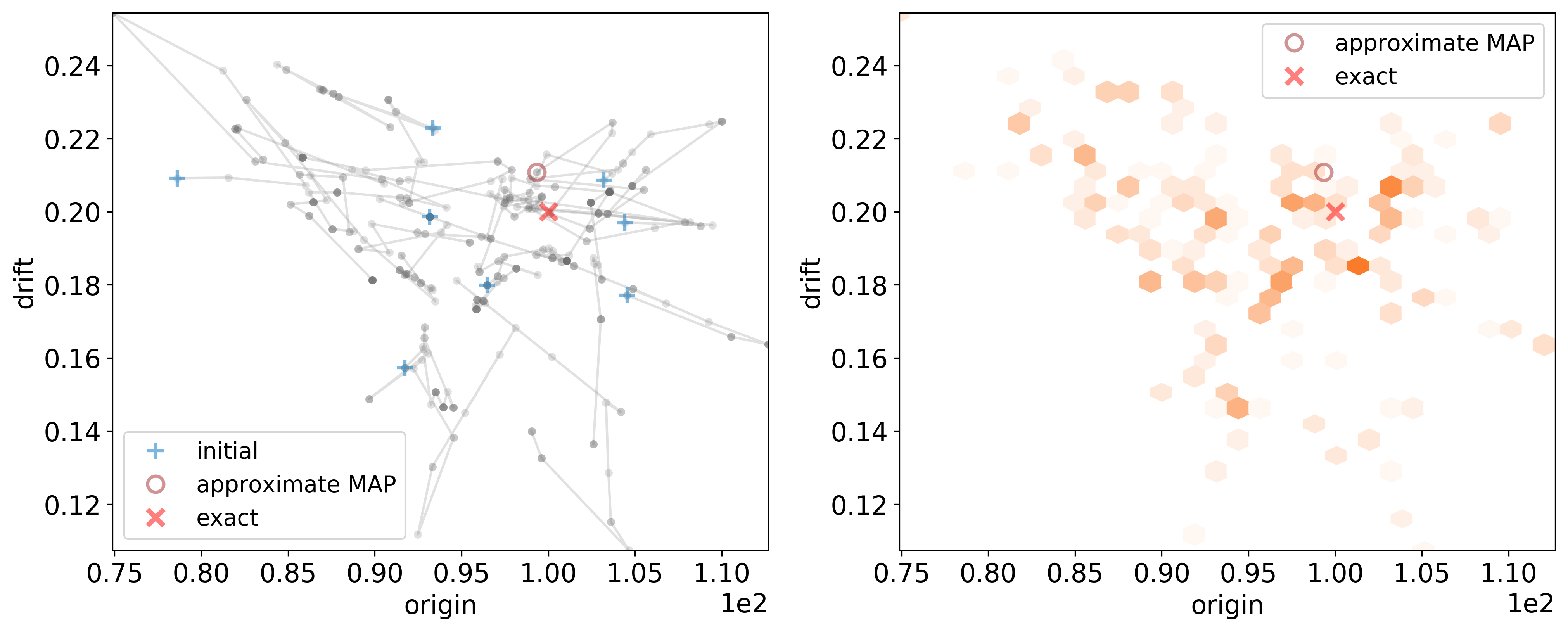
Joint pairwise marginal posterior distribution of origin and drift, including the corresponding Markov chains from the sampler. Legend: thin semi-transparent gray lines and dots - concurrent chains, orange hexagons - histogram of the joint pairwise marginal posterior parameters samples, blue “+” - initial parameters, brown “o” - approximate MAP parameters, red “x” - the exact parameters.
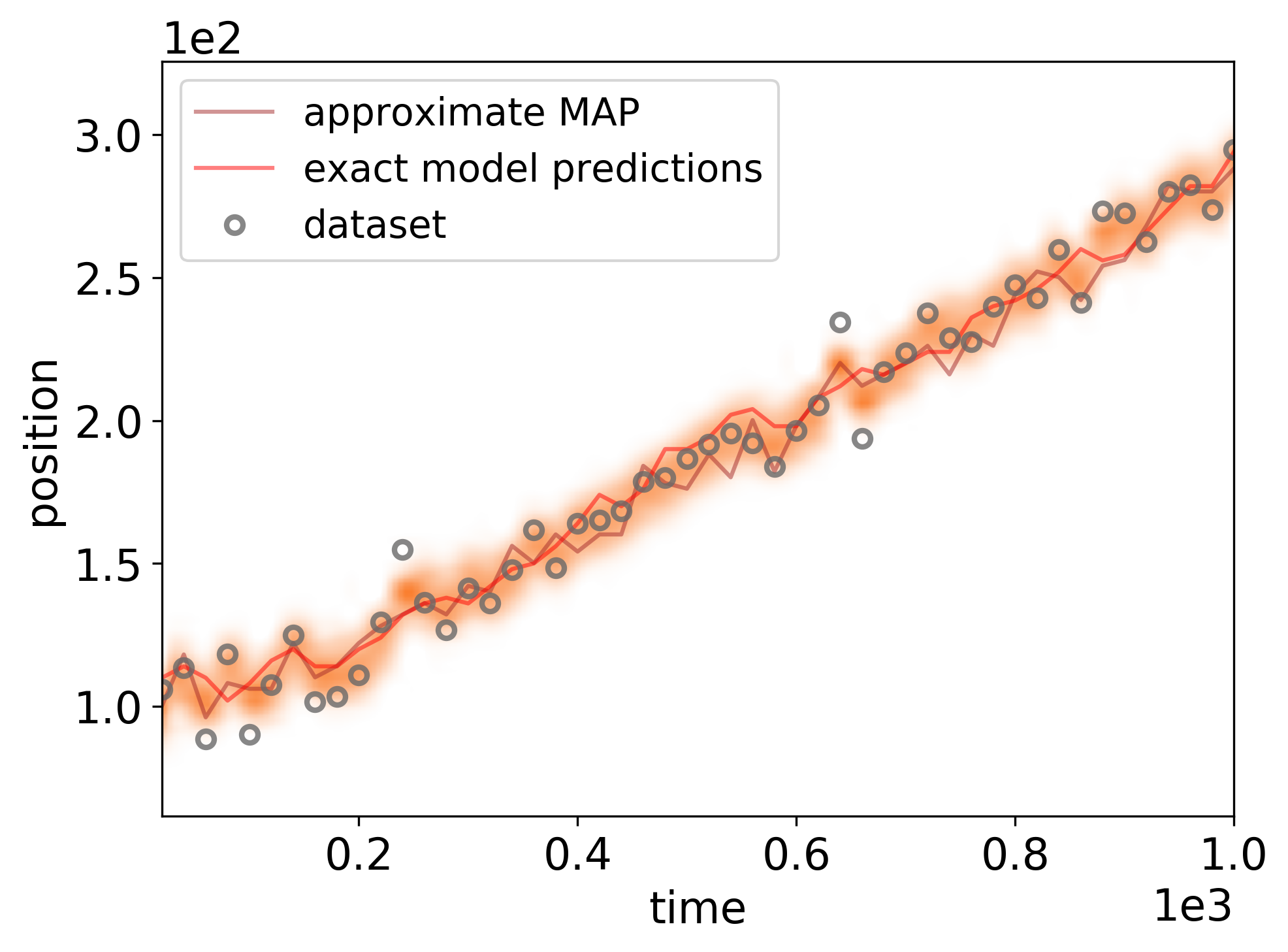
Posterior distribution of model predictions for the observational dataset. The shaded orange regions indicate the log-density of the posterior model predictions distribution at the respective time points, the brown line indicates the approximate MAP model prediction., the red line represents the exact model prediction values.

Quantile-quantile distribution comparison between the prediction residuals and the specified error model.
In addition to the plots in the fig directory, the auxiliary report directory is also updated,
appending information regarding
the approximate maximum a posterior parameters values (in report/randomwalk_MAP.txt):
==============================================
Maximum A Posteriori (MAP) estimate parameters
==============================================
$\sigma$ | drift    | origin
-------- + -------- + --------
9.24e+00 | 1.95e-01 | 9.78e+01
==============================================
and various metrics for inference efficiency (in report/randomwalk_metrics.txt):
==================================================================================================
Metrics for the inference efficiency.
==================================================================================================
Metric                                    | Value
----------------------------------------- + ------------------------------------------------------
Maximum A Posteriori (MAP) estimate       | batch:52, chain:2, sample:418, log-posterior:-2.01e+02
Multivariate Effective Sample Size (mESS) | not implemented
Multivariate thin period                  | not implemented
Univariate Effective Sample Size (ESS)    | 1 - 125 (across chains), with average 17 and sum 140
Univariate thin period                    | 1 - 71 (across chains), with mean 44
==================================================================================================
As with the plot_config.py script, at the end of the plot_results.py script
all generated plots are compiled into a LaTeX report under directory latex.
SPUX performance
The table of inference runtimes is available in report/randomwalk_runtimes.txt:
=================================================================
Runtimes (excl. checkpointer)
=================================================================
Timer                              | Value
---------------------------------- + ----------------------------
Total runtime (excl. checkpointer) | 2 hours 43 minutes 2 seconds
Average runtime per sample         | 0 hours 0 minutes 10 seconds
Equivalent serial runtime          | 2 hours 43 minutes 2 seconds
=================================================================
Even without explicitly specifying informative = 1 in sampler.setup (...),
the informative output is enable for the first and the last sample batches.
This allows us to generate a simplified and a standard timestamps plots,
providing an inisight into the runtimes profiles of the very last sample.
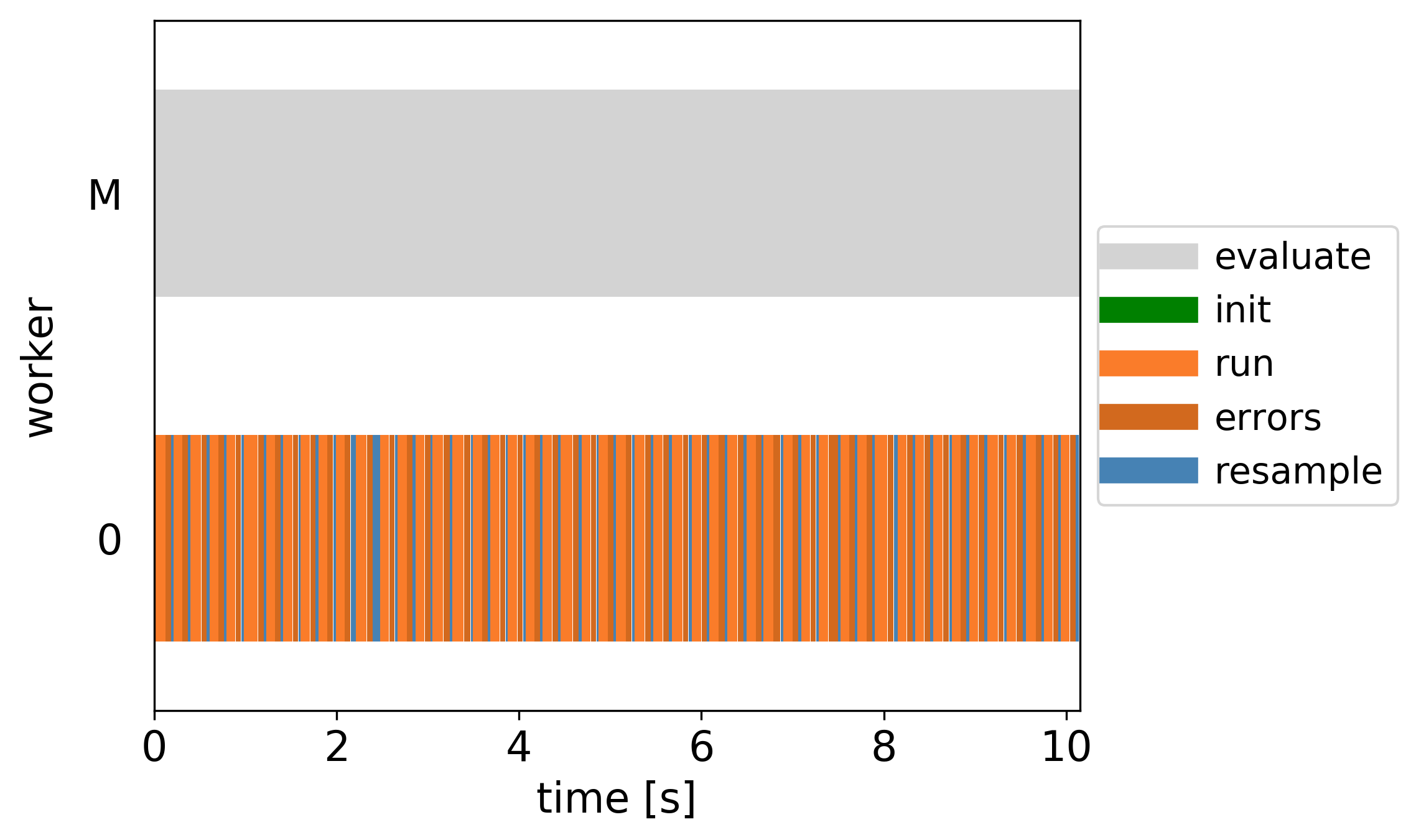
Timestamps of key methods within a single estimation of the PF likelihood across all parallel workers.
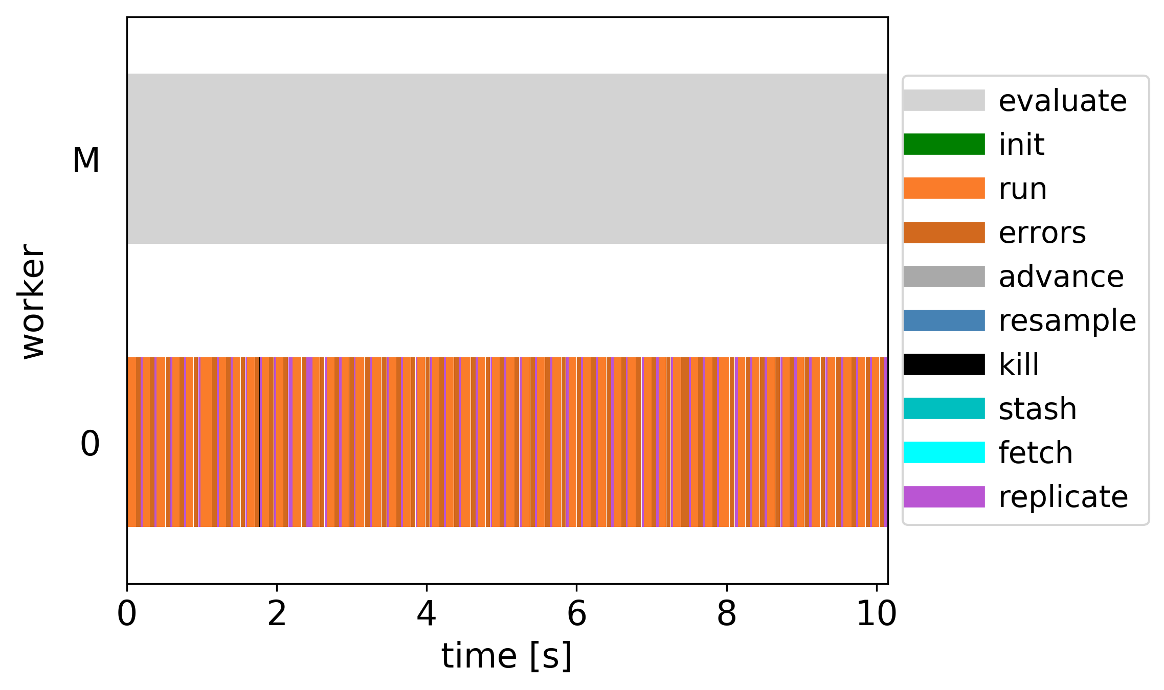
Timestamps of key methods within a single estimation of the PF likelihood across all parallel workers.
Continue sampling
It is possible to continue the sampling process where it finished without any additional re-evaluation of the likelihoods,
since all the needed information is already available.
The easiest way to continue sampling is to increase the number of samples as needed
and then execute the sampling script with the additional command line option --continue, for example:
$ python script_serial.py --continue
This automatically loads the most recent pickup file (see above).
An alternative and a more flexible way to manually customize the sampler.setup (...) method by providing
- sample batch
index- from which to continue (usually incremented last sampled batch index), feedback- from the previous sample batchindex(only forPFlikelihood),
and the sampler.init (...) method by providing (for the sampele batch index specified above)
initialparameters - respective loaded parameter samples for each sampler chain,posteriors- the posteriors of the above parameters.
An example of such advanced manual continuation script is available at examples/randomwalk/script_serial_continue.py.
Informative output
By default, the computation performance measurements
and the additional infos from each SPUX component
are incorporated into infos-*.dat for the first and the last sample batches.
Alternatively, you can choose to enable or disable such informative output
by setting informative = 1 or informative = 0 flag in the sampler.setup (...).
Note, however, that informative = 1 results in an overhead for your inference,
and is only advised for the non-production runs during the development stages.
You can then use the sample script
examples/randomwalk/plot_performance.py
to generate plots for timings and scaling for each sample batch,
in addition to the timings plots generated by plot_results above.
Profiling
If you would like to have more detailed information about the execution process,
you can enable the profiling by setting profile=1 in sampler.sample (...).
The profiling information after the execution of the framework will be saved in output/profile.pstats.
You can then use the sample script
examples/randomwalk/plot_profiler.py
to generate a report and a callgraph plot, which will be saved under the fig/ directory.
Randomwalk (parallel)
With minimal effort, the above example configuration could be parallelized either on a local machine or on high performance computing clusters.
Note, that NO MODIFICATIONS are needed for this particular Randomwalk model class.
For a more detailed discussion for other user-specific models written not in pure Python, refer to Customization.
SPUX executors
To enable parallel execution, each SPUX component in the main configuration script script.py
can be optionally assigned a parallel executor, specifying the number of parallel workers (for that particular component).
In this example, we use a separate script
examples/randomwalk/script_executors.py:
# === SCRIPT with SPUX components

from script import likelihood, sampler

# === EXECUTORS

# import required executor classes
from spux.executors.mpi4py.pool import Mpi4pyPool
from spux.executors.mpi4py.ensemble import Mpi4pyEnsemble

# create executors with the specified number of parallel workers and attach them
likelihood.attach (Mpi4pyEnsemble (workers=2))
sampler.attach (Mpi4pyPool (workers=2))

# display resources table
sampler.executor.table ()
The additional lines at the end of the script regarding the table estimate the needed computational resources,
which are determined by the number of workers requested in each executor.
Note, that a separate core is used for the manager process of each executor.
The table with estimated computational resources can be printed to the terminal simply by executing this script
(parallel inference is NOT launched at this point):
$ python script_executors.py
An example output of such table (for this particular configuration) is provided below, where the cumulative number of 31 cores are needed (bottom left cell, scroll horizontally to see everything).
============================================================================================
Required computational resources
============================================================================================
Component  | Class      | Task       | Executor | manager | workers | resources | cumulative
---------- + ---------- + ---------- + -------- + ------- + ------- + --------- + ----------
Model      | Randomwalk | -          | -        |       0 |       1 |         1 |          1
Likelihood | PF         | Randomwalk | Serial   |       0 |       1 |         1 |          1
Sampler    | EMCEE      | PF         | Serial   |       0 |       1 |         1 |          1
============================================================================================
Launching parallel SPUX
To launch a parallel inference using SPUX with the attached parallel executors as above,
we use a separate script for parallel runs which additionally initializes a parallel connector
and passes it to the sampler.executor.init (...), as given in
examples/randomwalk/script_parallel.py:
# === CONNECTOR INITIALIZATION

from spux.executors.mpi4py.connectors import utils
connector = utils.select ('auto')

# === SAMPLER with attached executors

from script_executors import sampler

# === SAMPLING

# SANDBOX
# use fast tmpfs
from spux.utils.sandbox import Sandbox
sandbox = Sandbox (path = None, target = '/dev/shm/spux-sandbox')

# SEED
from spux.utils.seed import Seed
seed = Seed (8)

# init executor
sampler.executor.init (connector)

# setup sampler
sampler.setup (sandbox = sandbox, verbosity = 2, seed = seed, lock = 50, thin = 10)

# init sampler (use prior for generating starting values)
sampler.init ()

# generate samples from posterior distribution
sampler (12)

# exit executor
sampler.executor.exit ()
Note the initialization of the connector as the very first item in the script. We emphasize, that such ordering of the connector and remaining SPUX components is mandatory to ensure efficient startup.
Assuming you have MPI installed (see Installation), the above script can be executed with:
$ python script_parallel.py
Note, that this is the shortest way to run it, but not the best. In particular, if the simulation crashes, the backtrace of the crash source will be complicated and the parallel processes cleanup will not be as desired. Hence, please consider using a more extensive command for production runs:
$ mpiexec -n 1 python -m mpi4py script_parallel.py
Note, that any needed additionally required MPI processes will be spawned automatically according to the resource table above,
hence for this configuration always use -n 1, independently of the workers in executors.
When script_parallel.py is executed, the computational resources table described in the preceding section
is printed to the terminal and also written to report/randomwalk_resources.txt.
Remark on MPI libraries
Note, that different MPI libraries provide different implementations, which have different configuration capabilities and might not completely follow the MPI standard.
Here we try to provide a list of useful advices to address any issues that you could encounter.
For OpenMPI (launched with mpirun or mpiexec):
- Specify
--mca mpi_warn_on_fork 0to avoid annoying warnings (only forSpawnconnector). - Specify
--mca pmix_server_max_wait 3600and--mca pmix_base_exchange_timeout 3600to avoid connection failures (not relevant forLegacyconnector). - For local testing, specify
--oversubscribeto use more MPI ranks than you have cores.
For CrayMPI (launched with srun):
- Specify
--hint=nomultithreadand--cpu-bind=rank.
Remark on executors
Note, that multiple serial (Serial) and parallel (Pool/Ensemble) executors
can be freely selected (that is, serial or parallel) for every SPUX component (Model, Likelihood, Sampler, etc.).
This freedom to use individual parallel executors of arbitrary size for every SPUX component provides a lot of flexibility, but also leaves ample of space for computationally inefficient parallel configurations. Hence, for large production runs, we strongly advice to take the following guidelines into consideration (decreasing in priority):
- Allocate most workers to the executors of the outer-most SPUX component(s) (e.g.
sampler). - Avoid parallel executors with few workers (less than 4) - replace them with
Serialexecutors.
SPUX will report the percentage of the number of manager cores w.r.t. the total number of all (manager and worker) cores. If the above guidelines are not properly implemented, this fraction could be larger than 20%, in which case SPUX will display an explicit inefficiency warning. Such warning will be skipped for jobs that requested not more than 8 cores in total, to filter out local debug and development runs, where parallelization efficiency is not of the highest importance.
Remark on connectors
The default way of initializing a connector is given by
from spux.executors.mpi4py.connectors import utils
connector = utils.select ('auto')
checks how many MPI ranks are available in MPI_COMM_WORLD intra-communicator
and automatically selects Spawn connector if only one rank is found (and all other workers need to be spawned.)
Since some HPC systems do not allow dynamically spawning new MPI processes, to run SPUX in parallel on 21 cores with MPI, simply execute:
$ mpiexec -n 21 python -m mpi4py script_parallel.py
Note, that -n 21 MUST match the total amount of required resources (bottom right cell) reported by running
examples/randomwalk/script_executors.py:
and stored in report/randomwalk_resources.txt.
In this case,
more than one MPI rank is available in MPI_COMM_WORLD intra-communicator,
and hence the Split connector is automatically selected.
Some HPC systems not only disallow dynamically spawning new MPI processes,
but also do not support modern dynamical MPI process management features such as inter-communicator creation
between two existing MPI intra-communicators using MPI_Comm_accept () and MPI_Comm_connect () methods.
In this case, you will simply need to use a legacy Legacy connector
instead of the Split connector.
Any such specific connector can be also specified manually either by replacing auto with spawn/split/legacy
in the connector initialization, or by specifying such connector name as a command line argument to the script_parallel.py, for example:
$ mpiexec -n 21 python -m mpi4py script_parallel.py --connector legacy
Remark on replicates
For parallel runs with replicate datasets (e.g. randomwalk-replicates example),
the Replicates likelihood performs guided load balancing
by evaluating the lengths of the associated datasets together and sorting likelihood evaluations,
taking into account adaptive number of particles in the PF likelihood as well, if used.
Higher priorities are assigned to the likelihoods with longer datasets and large number of particles (if applicable),
and lower priorities are assigned to the likelihoods with shorter datasets and smaller number of particles (if applicable).
If needed, one can disable such behavior by setting sort=0
in the constructor Replicates (...).
We warn, however, that depending on the executor configuration,
disabling sorting (and hence reverting to non-guided load balancing)
might lead to inefficient parallelization.
Performance progress
The performance plots of the last sample from a parallel simulation are also generated with plot_results.py.
Additional highly technical parallel performance plots can be generated by executing plot_performance.py,
provided that informative = 1 was used in sampler.setup (...),
and provide a summarized insight into the computation and communication balance within the parallel PF resampling stages,
over the evolution of the entire sampling process.
As with the plot_config.py and plot_results.py scripts, at the end of the plot_performance.py script
all generated plots are compiled into a LaTeX report under directory latex.
Parallel scaling
The template for post-processing results from multiple independent SPUX runs using a different cumulative amount of processor cores and generating the strong scaling plot is available in examples/randomwalk/plot_scaling.py.
Profiling (parallel)
Currently no special scripts for parallel profiling are packaged with SPUX.